Breaking All the Way Out – Techniques
by Maximilan Malek and Ralf Jung
"Breaking All the Way Out" was rendered with UberTracer, the raytracer we wrote during the course of this semester. To realize our short video, we implemented almost all of the optional assignments plus some more features we found out about through books or on websites, and which we considered interesting for our submission to the Rendering Competition. The most interesting of these features are described below.
To enlarge the screenshots, just click on the preview image.
Constructive Solid Geometry
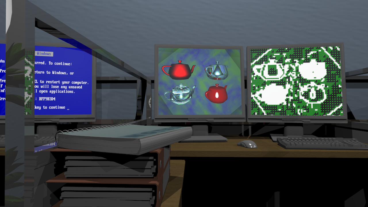
Constructive solid geometry was used to obtain the shapes used for the fog sample scenes (see the next section for screenshots), and for the plate of our small visual Escher quote of which you can find a screenshot on the right. The border of the plate is obtained by subtracting a sphere from a slightly larger one, and the intersection the remaining hull with an axis-aligned box to keep just a small belt.
We kept our implementation of CSG generic to avoid code duplication: The base class is able to compute any boolean set operation on volumes, so that the classes for intersection, union and difference only have to define how these operations behave on booleans. The actual algorithm is straight-forward: It queries the first intersection from both operands, and always keeps track of whether we are currently inside or outside the operands. As we assume the primitives used for CSG to be closed, the latter can be initialized by checking whether the first intersection found enters or leaves the object. Subsequently, the intersection that's closer to the origin of the ray is moved forward by computing the next intersection on the same ray, and the variable storing whether we are inside or outside this object is updated accordingly. If this changes the value of the boolean function defining the operation we are performing, we know that we just crossed the bounds of the CSG object, so an intersection is reported to the caller.
This algorithm sounds fairly inefficient when multiple CSG operations are nested.
The subvolumes are queried for intersections again and again.
For that reason, we first used another approach: The interface for primitives was enhanced with a function computing the list of all intersections on the given ray.
This drastically improves the (theoretical) computational complexity of intersecting deeply nested structures of CSG. However, it turned out that in our raytracer, this is actually
much slower than the naive appraoch we ended up using. Depending on the scene, the runtime was sped up by 20% to 80%.
We suspect that the reason for this is the overhead induced by memory allocation: To store the list of all intersections, memory has to be dynamically allocated while performing
the intersection test. For intersections with kD-trees, the resulting list of intersections also has to be sorted. Avoiding this overhead seems to vastly outperform
the lower complexity.
Fog
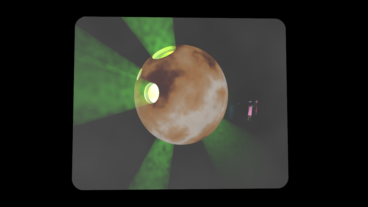
Fog is certainly one of the most important visual features of our demo - being able to visualize how the light is distributed in volumes (as opposed to the surface distribution) can create stunning visual effects. You can find some examples to the right.
The implementation mostly closely follows the lecture: After finding the (non-)intersection on a ray, we raymarch along the ray in small steps and sum up the contributions
of lights to all the points we visit. The weight is scaled down according to the density of the fog.
For heterogeneous fog (which you can see in the first image), we noticed that lots of time is spent computing the density of the ray from some intersection (or some point on a ray) to some light
source - which requires integrating the density over that ray. As these are secondary rays, and the result only influences how much light sources are weighted at a given point in the scene,
we decided that it's not worth spending so much computation time on these rays. Instead, we just compute the density on four points on the ray (in the center of each fourth of
the distance) and use that to approximate the total integral. This barely changed the visual appearance of the result, while drastically increasing rendering speed.
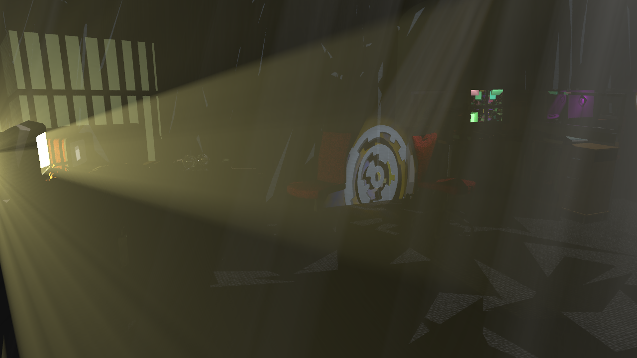
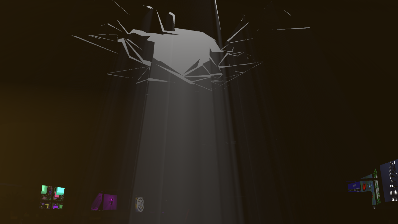
Bump Mapping
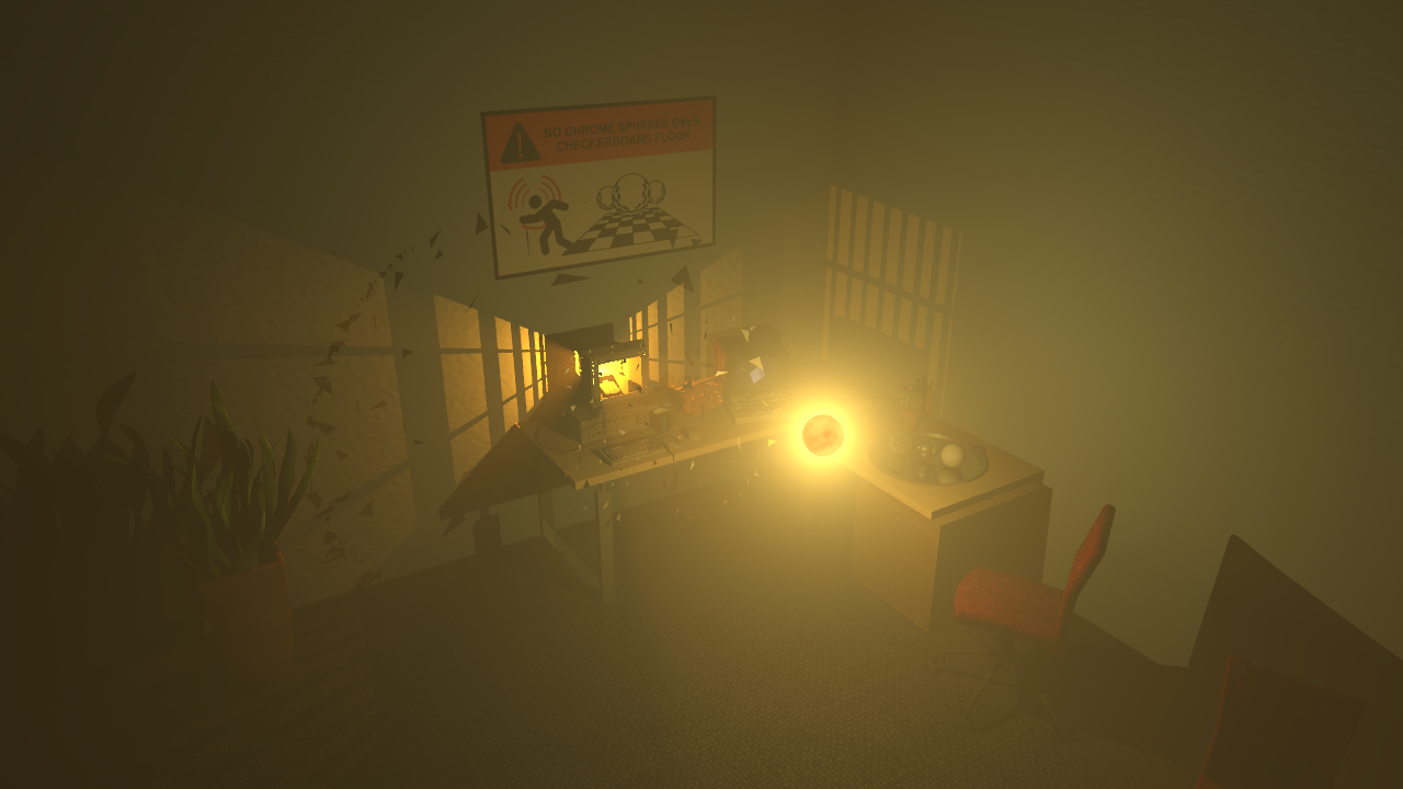
We used bumpmapping to give structure to the walls in our office. As you can see in the screenshot above, the noise on there is not just a texture: The black ("shadowed") parts of the bumps always point away from the light source (in this case, the fire in the screen). Compared to a flat wall, this made the office much more visually pleasing.
Implementation-wise, we went with the approach described in "Physically Based Rendering" instead of the one sketched on the assignment sheet, mostly because we found it easier to understand. To this end, we first compute the gradient of the displacement (as defined by the bumpmap texture) from the derivatives in u- and v-direction, in texture space. Then we need to compute the derivative of the displacement in u- and v-direction in the triangle we are bumpmapping, which is obtained by simply dot-multiplying the gradient with the base vectors of the triangle coordinates used for mapping triangle space to texture space. These are the vectors going from the first vertex to the second and third vertices. Finally, these derivatives are multiplied with the surface normal, scaled by the scaling factor, and added to the corresponding tangent vectors of the triangle to compute the displaced tangent vectors. Their cross product forms the normal used for shading.
We additionally also store the original (geometric) normal of the object. This is used to find out which light sources are above and which are below the currently lit surface. That way, we avoid some artifacts caused by shading normals not matching the actual geometry, like light bleeding onto a surface it cannot actually shine on.
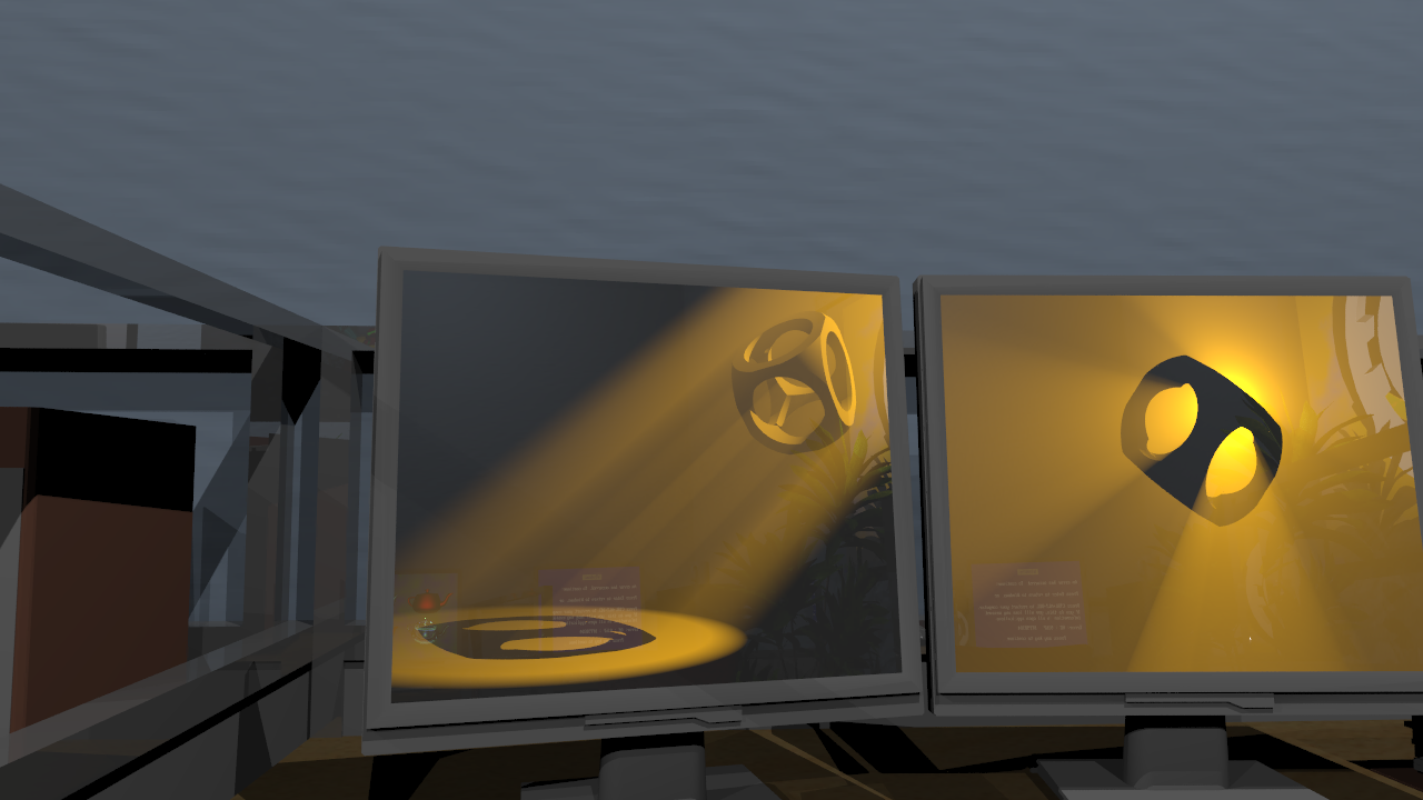
Adaptive Subsampling
Adaptive Subsampling can drastically increase the efficiency of rendering simple scenes. The basic idea is as follows: Instead of tracing a ray (or, in case of supersampling, several rays) for each and every pixel, only every eighth pixel on both dimensions is actually rendered. Then, for each of the resulting 8x8 pixel squares, a heuristic decides whether this square is supposed to be further subdivided or not. If the difference between the colors at the vertices is too large, the 8x8 block is subdivided into four 4x4 blocks, so five more rays are traced: One at the center of the block, and one at the center of each edge. This process is repeated until we arrive at 1x1 blocks, or until the color difference is considered small enough. The remaining pixels are then bilinearly interpolated.
Especially during construction of a scene, when surfaces are mostly untextured and hence relatively smooth, this technique is very efficient: While tracing only around ten to 20 percent of the rays, the important features of the image (edges of geometry and shadows) are typically captured well. As a result, we were able to use our raytracer as real-time editor for the scene.
The screenshot on the right shows the debug view of the subsampling renderer: When the scene shown on the left screen is rendered with subsampling, only the pixels shown in green and white are actually raytraced.
This adaptive subsampling approach is very much inspired by the subsampling in Heaven 7.
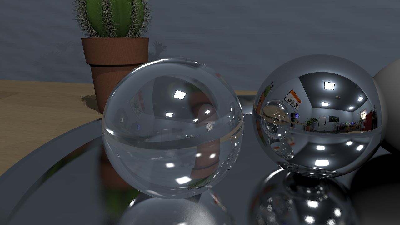
Gamma correction
All the color handling code in the ray tracer typically has a very fundamental assumption built in: That the color space we operate in is linear. To see this, consider the code adding up the contributions of all the light sources at a surface hit point. This "adding up" is done by simply summing of the RGB values of the contribution of each light source, which in turn is obtained by multiplying RGB values (namely, the color returned by the material BRDF and the light intensity). The assumption here is that a color value of 1 is twice as bright as a color value of 0.5, so adding up two lights of unit intensity results in a point twice as bright as it would be with just one light.
This assumption, however, is not actually true: PC screens will usually not display an RGB value of 1 twice as bright as an RGB value of 0.5. Instead, the monitor applies a gamma curve, which is typically (very close to) a power function of the input value: Given RGB intensity x, the voltage used to drive the corresponding pixel is proportional to xy. The value of y varies from screen to screen, but they are typically close to 2.2, so this value is often used in graphics.
Knowing this, the raytracer can compensate for this modulation to perform more realistic lighting computations. The ray tracing is defined to be carried out in linear color space.
Then, before the image is shown on screen or written to a file, we have to apply the inverse of the transformation done by the monitor, so that the final value
appearing on the screen is the one we originally computed. This is simply done by outputting x-y when the raytracer computed x.
Furthermore, we have to compensate for the fact that PNG files are already stored with this gamma correction in mind: In other words, the actually intended ratio of
brightness within an image is obtained by applying the gamma transformation in the raytracer. Hence, when a texture is loaded, we raise all color values to the
power of 2.2 to obtain the intended brightness.
Of course, there are other places where color information is fed into the raytracer, namely light sources and textures (like the constant texture). We decided that our raytracer does not automatically apply any gamma correction here. The reason for this is that this allows us to easily make a material or a light source twice as bright by simply doubling its RGB values. Also our color interpolation code (used to animate the color of light sources over time) automatically does the right thing: The brightness of the RGB components actually changes quadratic over time, thanks to the gamma correction performed on the final image. A user intending to use monitor-colors can simply perform the necessary transformation himself before feeding the values into the raytracer. We do naturally provide the corresponding convenience function in our color class.
More information about gamma correction can be found on Wikipedia and on the ACM SIGGRAPH Education Committee website.
Low Discrepancy Sampling
"Discrepancy" is a measure that describes how well a series is suited to numerically approximate an integral. In our raytracer, we implemented a sampler generating series of samples with low discrepancy, which means that less samples are needed to compute good-looking images (see the Wikipedia article for further information on these sequences). In particular, we implemented the (0, 2)-sequence described in "Physically Based Rendering", which is a series of points in a plane with the following remarkable properties: For any n, l1 and l2, the n samples starting at position n * 2l1 + l2 of the sequence are distributed in the unit square such that there is exactly one sample in each cell of an l1 by l2 grid. The samples for anti-aliasing, depth of field and the fuzzy mirror are drawn from such a series, and we ensure that the number of samples is always a power of two. This way, we capture more features of the functions these subsystems integrate over, than we would with pure random sampling. To avoid correlation between neighboring pixels, the sequences used for each pixel are scrambled with random values (for the details, see "Physically Based Rendering", chapter 7.4.3). This ensures we use an independent sequence for each pixel, while also guaranteeing that all pixels are covered with low discrepancy.
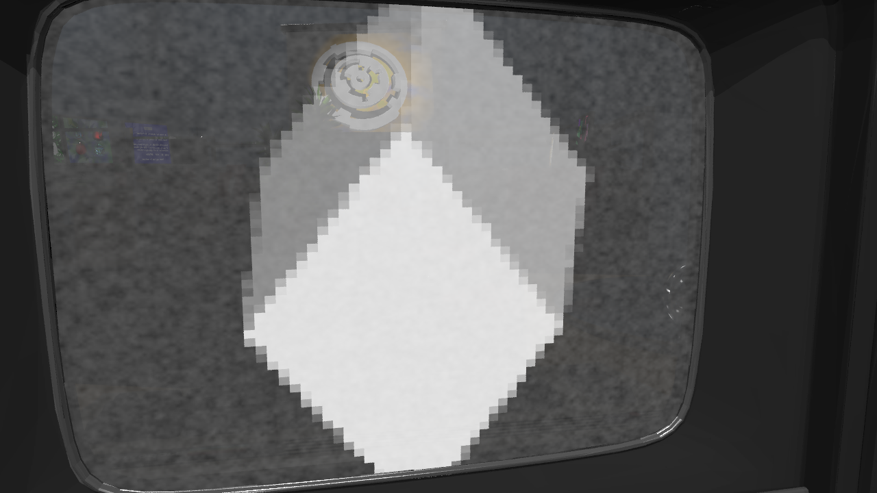
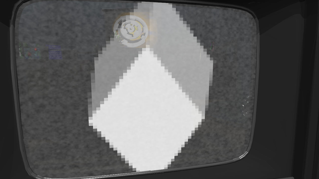
The two frames from our video to the right demonstrate the effect of low-discrepancy sampling for anti-aliasing: Both were rendered with 8 samples per pixel, but the first one used random sampling, while the second one employed the low-discrepancy sampling technique described above. Compare the right edge of the big-pixeled cube, and the white highlight at the bottom of the screen.
B-Splines
For most of the animation and moving objects, we used quadratic and cubic
B-Splines as described in the
Geometric Modeling lecture
by Tino Weinkauf et al.
B-Splines allow to interpolate smoothly between control points.
Cubic B-Splines guarantee no discontinuities in the first and second derivative, that means no sudden jumps in position,
velocity, or acceleration, which gives an overall smooth movement. This is especially useful for camera paths.
The control points can be of any dimension, and we used manually defined coordinates, angles, and colors as control points.
Examples include:
- Camera path (6D B-Spline for x, y, z, yaw, pitch, roll)
- Fireball movement
- Time modulation (slowmotion effect)
- Fire light colors
- Flickering when the room light turns on
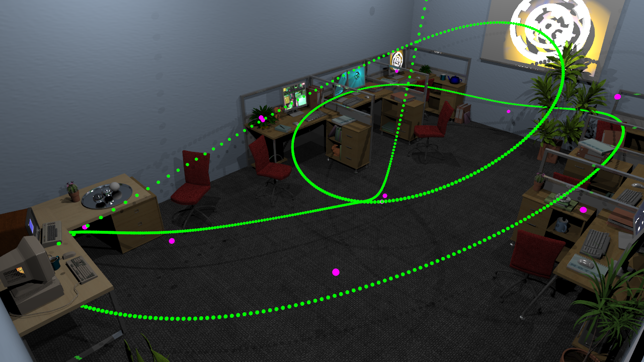
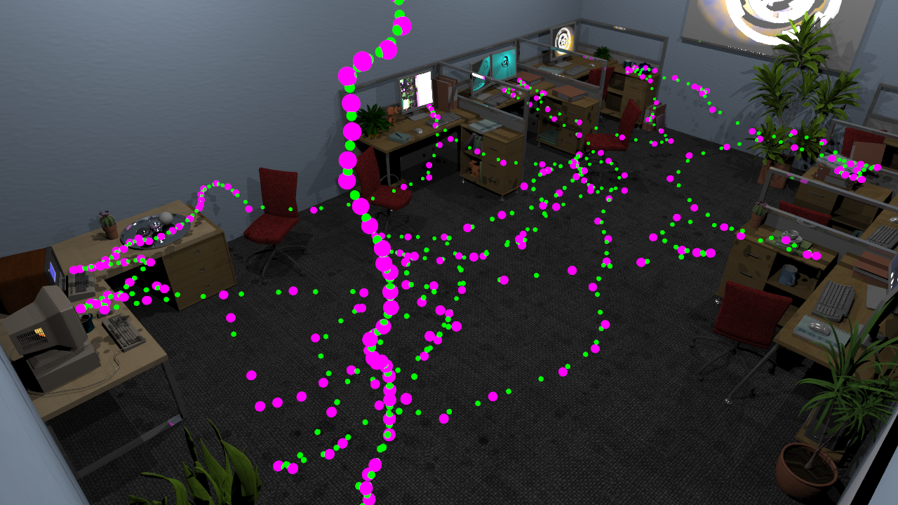
To the right, you can see a visualization of the B-Splines. The upper image shows the ball path, the lower image shows the camera path (the rotation cannot be visualized this way, though). Pink dots are control points, green dots are positions sampled along the resulting spline.
Triangle generation
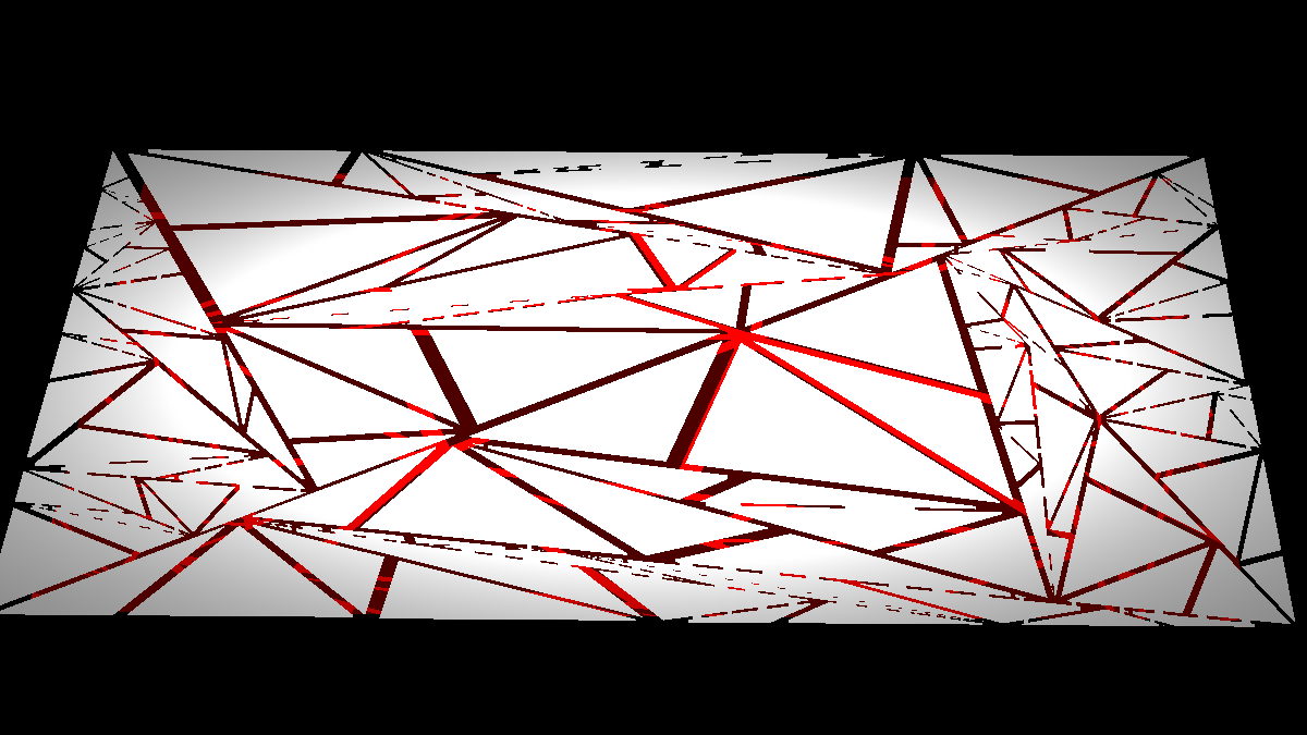
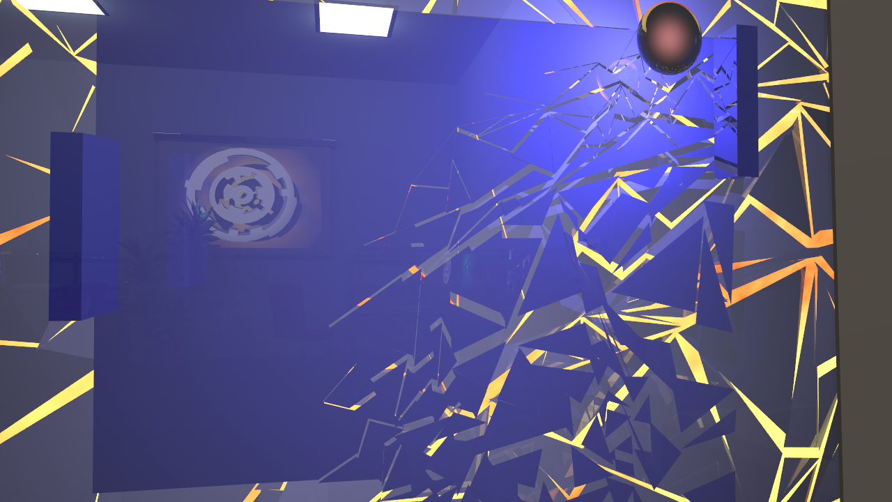
The splitters that remain of the pong playfield, screen glass, and the ceiling are automatically generated using a simple triangle splitting algorithm. Given a rectangular area, we create a fixed number of triangles exactly covering that area. This way, most of the scene is rendered with single quads, and only at the time the splitters are generated, the quad itself is removed from the scene. The (fake) physics are scripted in Lua and independently calculated for each triangle. There is no collision.
Progressive splittering is implemented by specifying an initial point (in case of pong, the lower right corner;
and for the ceiling, the position where the ball crosses it), from which each triangle's distance is calculated.
The initial physics update is delayed by a time proportional to that distance.
The triangle generation algorithm itself does not respect that point, all it uses is deterministic randomness.
Depth of Field
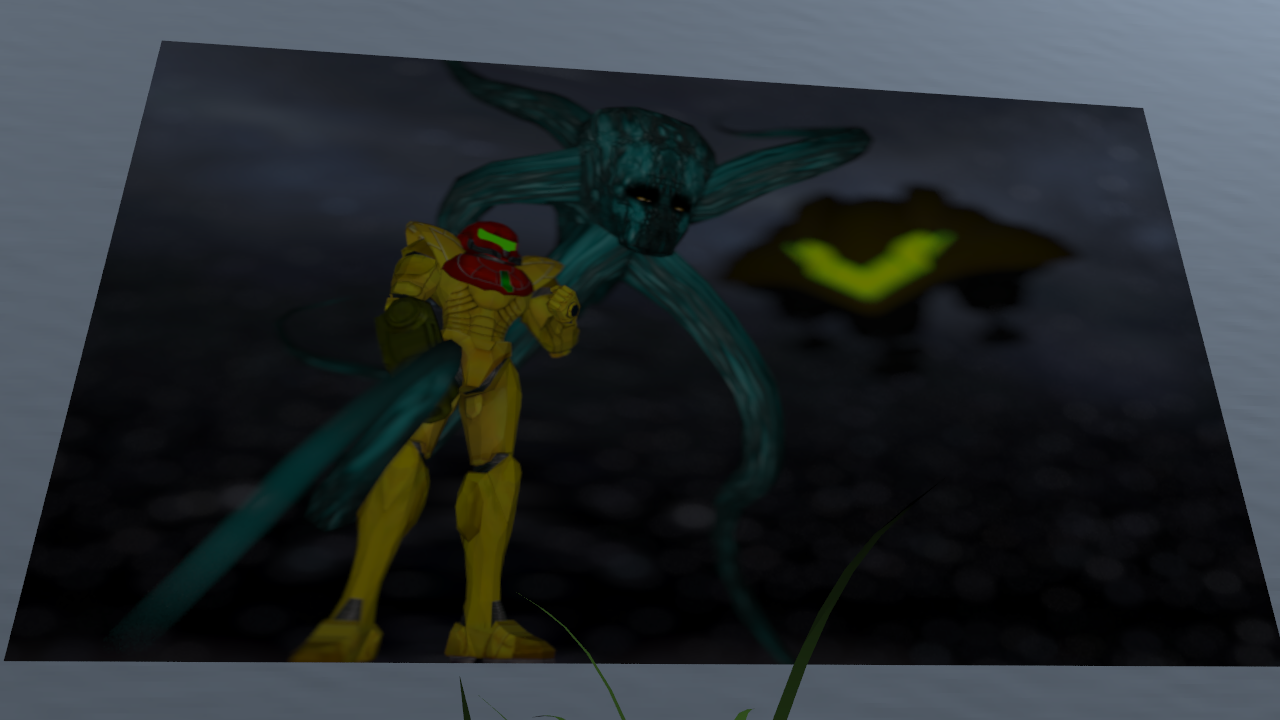
Our Depth-of-Field implementation is fairly standard. The only difference to the course reference is that we use Low Discrepancy Sampling to cover as much of the area displayed on a single pixel, as possible. The aperture samples used by the DoF camera for all the rays of a single pixel, are chosen from a low discrepancy sequence. A subtle complication arises when these samples are converted to coordinates on a disc: The standard technique we learned in the lecture redistributes the samples in a way that the low discrepancy is lost. Samples which were far apart in the [0, 1]2 square can be close together on the disc. Hence we implemented an alternative mechanism described in "Physically Based Rendering" (chapter 7) to convert uniform random samples to disc coordinates, in a way which preserves the low discrepancy.
In our video, we used Depth of Field to render the recursive subscene that is displayed on one of the posters at the wall.